WEEK FOUR
TOPIC:STATIASTICS
CONTENT
- Frequency Table.
- Cumulative Frequency Table.
- Histogram.
When data has a large number of values, it is cumbersome to prepare its frequency table; hence the data are organized into classes or groups to overcome this problem. E.g 0 – 4, 5 – 9, 10 – 14 e.t.c.
The range of the classes is first considered before we group the data. When data is divided into groups, it is called a grouped frequency distribution.
Grouped frequency distribution: The groups into which the data are arranged are called class intervals
e.g 15 – 19
Class Limit: The number of each class intervals is called class limits of that interval.
Consider the class interval 20 – 24,
20 = lower class limit, 24 = upper class limit
Class Boundaries: When data is given to the nearest unit, the class interval 34 – 37, has a lower class boundary of 33.5 and upper class boundary of 37.5.
Consider the intervals below: 20 – 24, 25 – 29 ETC. To obtain the class boundaries of 25 – 29,
24 + 25 = 24.5, 29 + 30 = 29.5
2 2
Class Width: This is the difference between the upper class boundary and the lower class boundary.
Class Marks: This is the centre or mid-point of any class interval. It is obtained by finding the average of the lower and upper limits. Find the class mark of the following class intervals 40 – 44, 45 – 49, 50 – 54 etc.
| Class Interval | Class Mark |
| 40 – 44 | 40 + 44 = 42 2 |
| 45 – 49 | 45 + 49 = 47 2 |
Cumulative Frequency Table:
This is the table that shows the cumulative frequency of each of the classes and it is the running total of the frequencies class by class, giving the total frequency.
EXAMPLE: In a mock examination for the final year Chemistry class, the following were obtained by 50 students.
71 63 70 45 59 82 61 79 37 89
33 56 39 42 64 73 59 67 72 60
46 36 61 87 91 67 54 72 39 43
57 65 45 52 35 46 64 37 95 86
76 73 67 71 74 82 61 59 58 43
Using class interval 31 – 40, 41 – 50 … e.t.c Construct a table showing the following columns: class interval, class boundary, class mark, frequency and cumulative frequency.
| Class interval | Frequency | Class boundary | Class mark | Cumulative Frequency |
| 31 – 40 | 6 | 30.5 – 40.5 | 35.5 | 6 |
| 41 – 50 | 9 | 40.5 – 50.5 | 45.5 | 6 + 9 = 15 |
| 51 – 60 | 9 | 50.5 – 60.5 | 55.5 | 9 + 15 = 24 |
| 61 – 70 | 11 | 60.5 – 70.5 | 65.5 | 11 + 24 = 35 |
| 71 – 80 | 9 | 70.5 – 80.5 | 75.5 | 9 + 35 = 44 |
| 81 – 90 | 4 | 80.5 – 90.5 | 85.5 | 4 + 44 = 48 |
| 91 – 100 | 2 | 90.5 – 100.5 | 95.5 | 2 + 48 = 50 |
EVALUATION
The following figures show how many people visited an art gallery each day for 50 days.
Using class interval 11 – 20, 21 – 30 … e.t.c Construct a table showing the following columns: class interval, boundary, class mark, frequency and cumulative frequency.
30 60 53 54 35 51 13 36 43 44
44 38 39 52 45 39 25 27 31 44
29 46 49 42 47 43 34 52 50 39
53 25 28 51 54 33 35 45 51 59
19 28 34 42 48 51 20 25 37 38
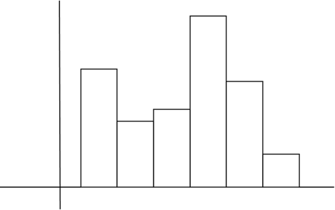
HISTOGRAM
This is a type of bar chart, each bar corresponding to one mark and with its length proportional to the frequency of that mark. The class marks or centres, class boundaries can be used on the variable scale. In histogram, the bars are joined together and must be of equal width, except when dealing with unequal class interval.
The following table shows the distribution of marks scored by a class of 80 students.
| Marks | 10 – 14 | 15 – 19 | 20 – 24 | 25 – 29 | 30 – 34 | 35 – 39 |
| Frequency | 18 | 9 | 11 | 25 | 14 | 3 |
Draw a histogram for the distribution.
Solution
| Class Interval | Class Mark | Frequency |
| 10 – 14 | 12 | 18 |
| 15 – 19 | 17 | 9 |
| 20 – 24 | 22 | 11 |
| 25 – 29 | 27 | 25 |
| 30 – 34 | 32 | 14 |
| 35 – 39 | 37 | 3 |

 25 –
25 –
20 –
15 –
10 –
5 –
0 9.5 14.5 19.5 24.5 29.5 34.5 39.5
Class boundaries
EVALUATION
Draw a histogram to illustrate the data shown below.
| Heights(cm) | 120 – 129 | 130 – 139 | 140 – 149 | 150 – 159 | 160 – 169 | 170 – 179 |
| Frequency | 6 | 15 | 31 | 37 | 9 | 2 |
GENERAL EVALUATION
1. Construct a table showing the following columns: class interval, class boundary, class mark, frequency ,and cumulative frequency for the distribution shown below.
| Shoe Sizes | 5 – 9 | 10 – 14 | 15 – 19 | 20 – 24 | 25 – 29 | 30 – 34 | 35 – 39 |
| No of students | 5 | 7 | 6 | 2 | 3 | 4 | 3 |
2. Draw a histogram for the distribution.
READING ASSIGNMENT
New General Mathematics SSS1, page 180, exercise 14e, numbers 2,3,4 and 7.
WEEKEND ASSIGNMENT:
1. The thickness of 20 samples of steel plate are measured and the results (in mm) to two significant figures are as follows:
7.3 7.1 6.6 7.0 7.8 7.3 7.5 6.2 6.9 6.7
6.5 6.8 7.2 7.4 6.5 6.9 7.2 7.6 7.0 6.8
Construct a table showing the following columns: class interval, class boundary, class mark, frequency and cumulative frequency, using class interval 6.2 – 6.4, 6.5 – 6.7 e.t.c
2. The following table shows the distribution of the masses of 120 logs of wood, correct to the nearest kg.
| Masses (kg) | 15 – 24 | 25 – 34 | 35 – 44 | 45 – 54 | 55 – 64 |
| Frequency | 14 | 54 | 24 | 26 | 2 |
- Draw a histogram for the distribution.